Toolkit Design

Information Flow

Genetic algorithms have a great many variations but also share common points. All have the common features of initialisation, evaluation, populations, and reproduction. From here that the design of the generic toolkit was started by considering the information pathways of the algorithm. However, this is insufficient because certain specialisations are not described in such a model. In particular there were three areas of deficiency. A large group of genetic algorithms use fitness functions to set up a more competitive environment. Most genetic algorithm make a considered opinion on whether to finish. Finally some genetic algorithms monitor their changing populations over time for historical tracing or additional processing, these are all specifically mentioned in the statement of requirements. Taking all these aspects into account produced Figure 6 which shows information steps within a generic genetic algorithm and the information flow between steps which typically consist of potential problem solutions. Those steps dealing with the three aspects which are not common to all algorithms are shown in grey.

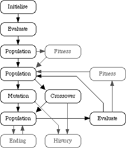
Figure 6 - Information flow

Toolkit Components

From the beginning of the project the intention had been to produce an object-oriented toolkit. Such a model is well suited to the desired extensible toolkit. Abstract classes would provide the toolkit and users inherit concrete classes for use in a particular genetic algorithm. This facility would also facilitate the construction of the toolkit enabling the range of services to be slowly expanded.

Primary in toolkit design was the notion of flexibility and the speed at which a new algorithm could be assembled. Even so this had to be balanced against implementations which would take an unacceptably long time to run. Several genetic algorithms suggested minor variations which did not fit in with the majority of other algorithms. For example the elitist breeding technique is an extension of the standard generational technique. No other similar behaviours are mentioned in the literature and so the toolkit would have to implement elitism separately and either flag if active or not for a particular algorithm. Such behaviour is contrary to the generic ideal and slows down many algorithms for benefit a few.

Fortunately a clue to the solution is already described, Lawrence Davis (1991). Two stages from the standard genetic model, the deletion of old individuals and insertion of new individuals, are often placed together. This suggested consolidating these procedures into a single object, one to do both jobs. A Model object would also take over most other stages of the genetic algorithm, its exact behaviour depending on the parameters such as reproduction operators but also on that model's particular make up.

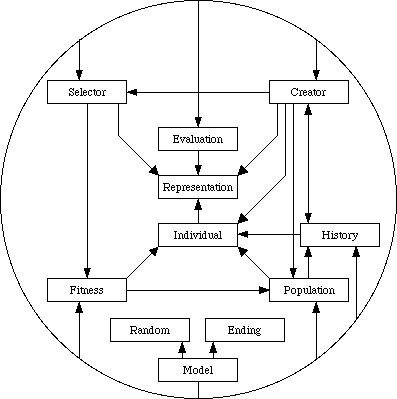
Figure 7 - Class dependencies

Figure 7 shows final choice of classes for the toolkit and the dependencies between them. Each arrow represents one class's knowledge about another. Around the diagram is a circle, this is just a combination of several dependency arrows. As can be seen the Model object has direct control over almost all other classes within the toolkit. Several objects have appeared in the diagram which do not seem to have any correspondence to the information flow diagram.

Random is a pseudo-random number generator to provide for the probabilities needed by a genetic algorithm. By using a single controllable generator for the algorithm experiments can be replicated. Simply by storing the initial random number seed and the parameters used by the genetic algorithm, the same results may be obtained again and again. If real or arbitrary random numbers were used every individual would have to be recorded and traced to provide the same service.

Representation is a abstract holding place for a single problem solution. Concrete examples of this class include binary vectors, ordered lists of integers, or 3D matrices. With all different representations packaged in the same way they may be dealt with equally by most of the toolkit. Only functions which depend on specific representations such as evaluation and reproduction operators need separate them.

Evaluation is apparently only a function and does not need object status. Simple evaluations can indeed be calculated directly from the representation but many need auxiliary information. An object provides storage space for such details, an example of such is shown in Chapter 5.

Individual is the encapsulation of a Representation. Each individual is uniquely identifiable not only within a single generation but within all generations in a particular algorithm. Even individuals with identical representations may be differentiated. Tracking the development of individuals over time is impossible without this. Population provides a simple set for storing individuals.

Ending makes the decision on whether or not another cycle of the genetic algorithm should be made. Several concrete class are available including ones based on time, generation count, and target evaluations. Complex combinations can be formed by joining simple ending objects with And, Or, or Xor operators also implemented as Ending objects.

Breeding Model

Model encompasses both breeding technique and major control of the genetic algorithm. All algorithms are to be dealt with in a uniform fashion and because of this the Model is sometimes burdened with additional work. Here is the final design used for this class formatted as - method: arguments > result:

ctor: Creator,population_size > Model
ctor: input_stream > Model
print: Model, output_stream
run: Model, Evaluation, Fitness, Selector, Creator, Ending
run: Model: Evaluation, Fitness, Selector, Creator, Ending, History
get_population: Model > Population

Two creator methods (ctor's) are used, either populating the model with newly created individuals or recovering individuals specified in an input stream. A complement to this is the print method which records the current status of the model for prosperity. The internal population may be accessed to obtain the result after the algorithm has finished. Most work is done by the run method which take several arguments, each specifies one aspect of the genetic algorithm. Two versions of run are present, one which takes a History object, the other does not. This is one example of where a decision has to be about generality and efficiency. Recording the births, deaths, and parentage information in a genetic algorithm will obviously take extra time. Hence two separate methods, only if this user requires the feature must the additional time be taken.

Other classes keep the work which must be done by the Model to a minimum implementing any single instance is not difficult. Here is an example of the run method from the Generational Model which is used by The Blues:

done := false;
while not done loop
  Attach(Fitness, Model.Population);
  Attach(Selector, Fitness);
  Create(Reproduction, population, population_size);
  Transfer(Model.Population, population);
  Done(Ending, done);
end loop;

Fitness Function

Fitness functions are applied after evaluation and before parent selection. An equivalent could also be used when removing individuals from the population but this is not a common feature. Evaluations of all individuals in the population must be presented to the fitness function so that comparisons can be made. One possibility is to in effect reevaluate each individual, assigning them this new value, and then carry to on as normal. Although easier to implement than other schemes this was rejected because it would destroy the initial evaluation which may be required again and could be expensive to calculate.

One solution is a wrapper around the Population class. A fitness object is passed into the genetic model and is then be attached to a given population. When attached the object calculates an associated fitness score once for each individual. To obtain fitness values a fitness iterator is created which moves through the population returning individuals and their fitnesses. A separate iterator is required so that multiple scans of the population can progress at the same time.

This created a small problem, The Blues does not need a fitness function but must have one because of the decision to apply the same methods to all genetic algorithms. Along with standard fitness function - Windowing, Linear Normalisation, and so on - another, the Unity Fitness class had to be introduced. For each individual in the population this returns the same value as found during evaluation. Null operations such as this are often not noticed within a system until a rigorous examination is made.

Parent Selector

From a fitness capped population individuals must be selected for reproduction. The obvious approach is an abstract Selector object and a number of concrete classes representing the different ways of choosing individuals. Common examples of selection techniques are best, random, and roulette wheel. The consistent approach to genetic algorithms required by the toolkit means others classes are needed. Some particular genetic algorithm prefer low values to high values. Normally one would change the evaluation function to invert values but in preference to that other selectors can be used lowering the burden on the algorithm's implementor. For example an Anti-roulette Wheel Selector returns individuals with a probability inversely proportional to its evaluation. If this class replaced the Roulette Wheel Selector in The Blues then black would become the preferred colour. Implementing selectors as objects also gives some speed advantages. When attached to a population any necessary calculations to make the selection can be done once and only once. For example in the instance of a best individual selector one single search for this individual is made and the result can then be recorded. Any future calls to the selector will produce the same individual instantly.

Individual Creator

Creator class combines both initialisation and reproduction. Original designs had included two separate class but these were merged in an effort to reduce the complexity of the toolkit. Both perform similar jobs, the production of new individuals, and so have similar requirements. Initialisation at the start of a genetic algorithm in the standard case does not normally require parent individuals to draw on. Some genetic algorithms start with a population of specialised individuals who have been generated in other genetic algorithms. Initialisation becomes a matter of cloning old individuals into the new population. Equally, although reproduction normally involves parents, some algorithms may occasionally introduce completely new individuals to keep up genetic diversity.

Given that several reproduction operators are used in each genetic algorithm a mechanism must exist to choose between them. One possibility was to pass in a set of reproduction operators for each run of the genetic algorithm. Associated with each is a weight determining the probability of that operator being chosen. A more advanced technique categorises reproduction operators as to whether or not they are combined operators. That is whether they just mutate or whether they mutate then crossover individuals. Repair algorithms can also be implemented as combination operators. First the normal reproduction operator is applied and then the resultant individual is corrected of any defects, converted back into a legal representation. This technique was chosen and implemented using a tree structure. A single combined reproduction operator is passed into the Model which would execute the appropriate leaf operators. Shown in Figure 8 are special And, Or, and Xor operators which form internal nodes. This reproduction is one but not both of (both Crossover and Mutate) or (either Crossover or Mutate or both). Both and Xor class hold weights to determine the probability of each branch of the tree being chosen.

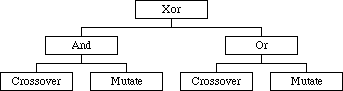
Figure 8 - Reproduction tree

Some implementation issues have to be resolved. The problem of getting information from the selection operator to one or more reproduction leaves. One solution was to give each operator its own selector during initialisation, some attached to the population through the fitness class and others attached to sibling reproduction operators. Figure 9 shows selectors as arrows pointing towards their source. The population class is represented by small grey circles. Such a design would treat all creation events evenly whether they draw from the old population or another operator. Each stage would have to create complete individuals ready to pass on to another operator and this would slow the algorithm. Also the ancestry of an individual might get a little chaotic with some parents never existing in any population.

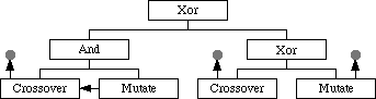
Figure 9 - Multiple selectors

The final solution was for the reproduction tree to be informed of its selector and this information propagated down the tree to all reproduction operators who required it. During a creation event control was provided through the combination operators. The And operator will have to pull individuals from the selector and pass them first to its left hand operator and receiving solution representations but not individuals, these bare representations are then passed to the right hand operator, changed and returned before begin packaged as individuals. The Xor operator can determine the relevant sub-tree and pass control down. The Or operator must decide to use either one or both sub-trees and can then act like an Xor or And operator respectively.

Several methods are required to implement this technique.

create: Creator, Population, size
create: Creator, History, Population, size
parents: Creator > number
breed: Creator, [Representation], Representation > succeed

When the Model object require more individuals the create method is called. Two variants were provided, one to keep track of ancestry, the other not. Combination operators use the parents method to plan their strategy. Finally the breed method produces new representations which could then be wrapped up as individuals after more modification.

A question never adequately answered during the design of the toolkit is how many individuals should a crossover produce. Classic genetic algorithms set the answer at two, or for some of the more complex crossover, a larger but fixed number. Creating multiple individuals did not mesh with the toolkit's generality. When asking for a single individual a crossover might be selected from the tree and that would produce two or more individuals instead. The toolkit could not know how many to expect and would not know what to do with any surplus. The chosen solution was to only ever create a single individual for any reproduction operator. More operations might have to be performed but there can be no confusion about the number of individuals produced and no time wasted on creating surplus individuals.